Charge Stations

Our Mission

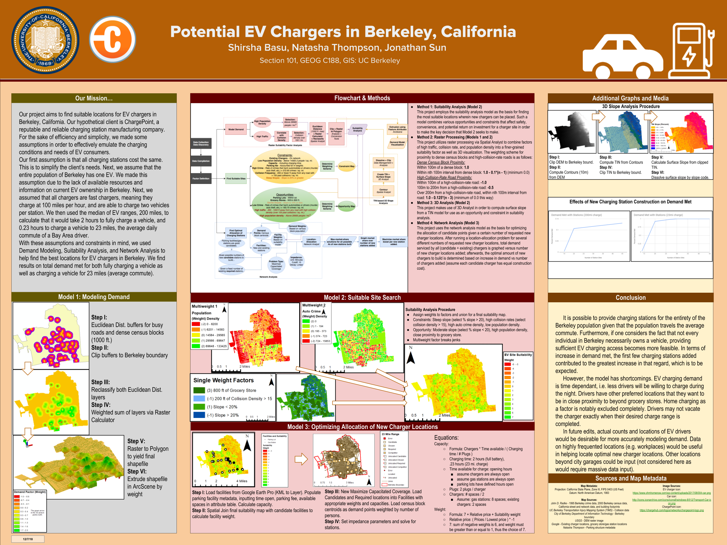
Our project aims to find suitable locations for EV chargers in Berkeley, California. Our hypothetical client is ChargePoint, a reputable and reliable charging station manufacturing company. For the sake of efficiency and simplicity, we made some assumptions in order to effectively emulate the charging conditions and needs of EV consumers. Our first assumption is that all charging stations cost the same. This is to simplify the client’s needs. Next, we assume that the entire population of Berkeley has one EV. We made this assumption due to the lack of available resources and information on current EV ownership in Berkeley. Next, we assumed that all chargers are fast chargers, meaning they charge at 100 miles per hour, and are able to charge two vehicles per station. We then used the median of EV ranges, 200 miles, to calculate that it would take 2 hours to fully charge a vehicle, and 0.23 hours to charge a vehicle to 23 miles, the average daily commute of a Bay Area driver. With these assumptions and constraints in mind, we used Demand Modeling, Suitability Analysis, and Network Analysis to help find the best locations for EV chargers in Berkeley. We find results on total demand met for both fully charging a vehicle as well as charging a vehicle for 23 miles (average commute).

Flowchart and Methods

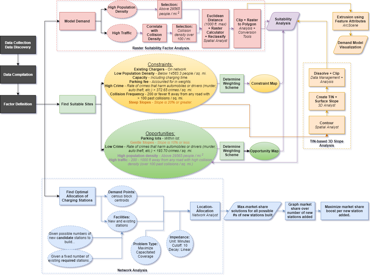
Method 1: Suitability Analysis (Model 2)

This project employs the suitability analysis model as the basis for finding the most suitable locations wherein new chargers can be placed. Such a model combines various opportunities and constraints that affect safety, convenience, and potential return on investment for a charger site in order to make the key decision that Model 2 seeks to make.

Method 2: Raster Processing (Models 1 & 2)

This project utilizes raster processing via Spatial Analyst to combine factors of high traffic, collision rate, and population density into a finer-grained suitability factor as well as 3D visualization. The weighting scheme for proximity to dense census blocks and high-collision-rate roads is as follows:

Dense Census Block Proximity:

• Within 100m of a dense block: 1.0
• Within nth 100m interval from dense block: 1.0 - 0.1*(n - 1) (minimum 0.0)

High-Collision-Rate Road Proximity:

• Within 100m of a high-collision-rate road: -1.0
• 100m to 200m from a high-collision-rate road: -0.5
• Over 200m from a high-collision-rate road, within nth 100m interval from road: 1.0 - 0.125*(n - 3) (minimum of 0.0 this way)

Method 3: 3D Analysis (Model 2)

This project makes use of 3D Analyst in order to compute surface slope from a TIN model for use as an opportunity and constraint in suitability analysis.

Method 4: Network Analysis (Model 3)

This project uses the network analysis model as the basis for optimizing the allocation of candidate points given a certain number of requested new charger locations. After running a location-allocation problem for several different numbers of requested new charger locations, total demand serviced by all (candidate + existing) chargers is graphed versus number of new charger locations added; afterwards, the optimal amount of new chargers to build is determined based on increase in demand vs number of chargers added (assume each candidate charger has equal construction cost).

Model 1: Modeling Demand

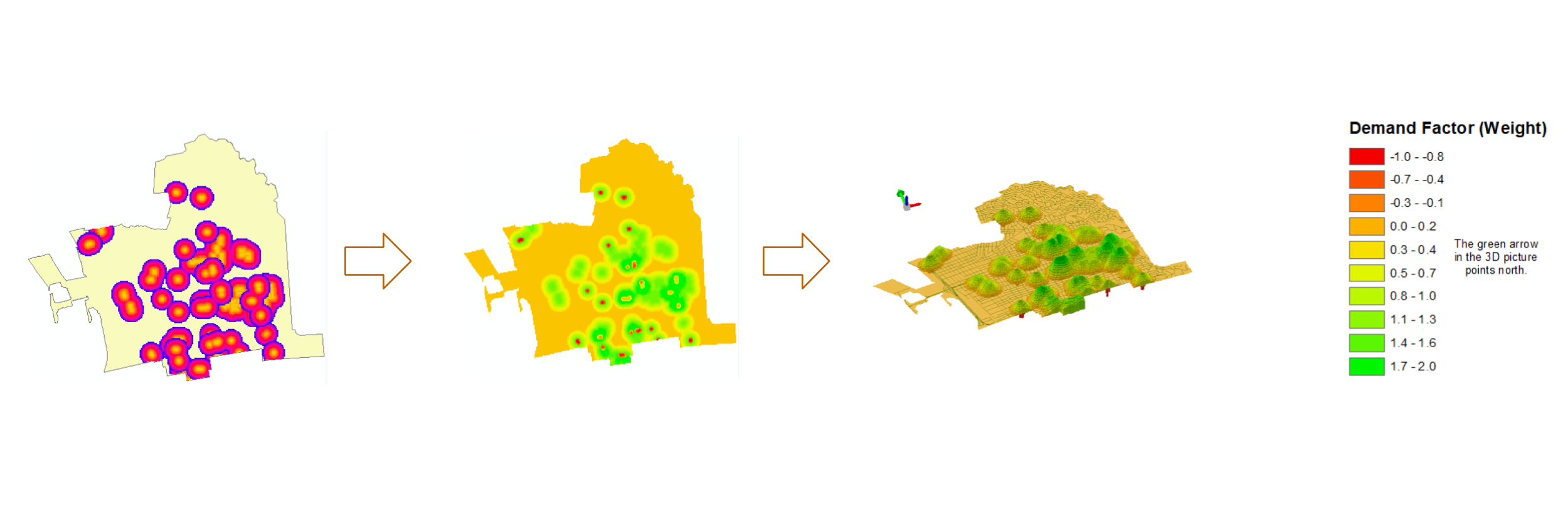
Step I: Euclidean Dist. buffers for busy roads and dense census blocks (1000 ft.).

Step II: Clip buffers to Berkeley boundary.

Step III: Reclassify both Euclidean Dist. layers.

Step IV: Weighted sum of layers via Raster Calculator.

Step V: Raster to Polygon to yield final shapefile.

Step VI: Extrude shapefile in ArcScene by weight.

Model 2: Suitable Site Search

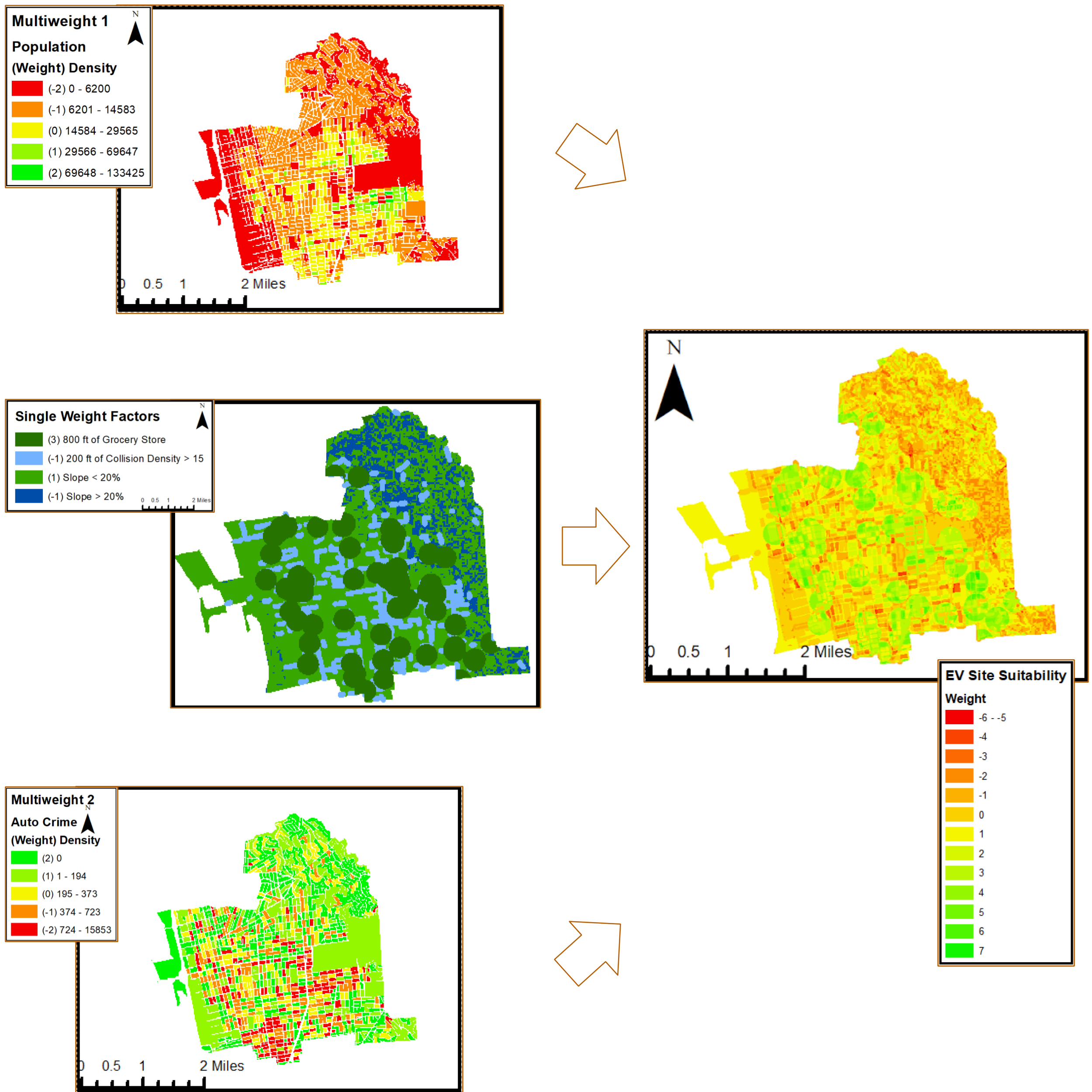
Suitability Analysis Procedure

• Assign weights to factors and union for a final suitability map.
• Constraints: Steep slope (select % slope > 20), high collision rates (select collision density > 15), high auto crime density, low population density.
• Opportunity: Moderate slope (select % slope < 20), high population density, close proximity to grocery store.
• Multiweight factor breaks jenks.

Model 3: Optimizing Allocation of New Charging Locations

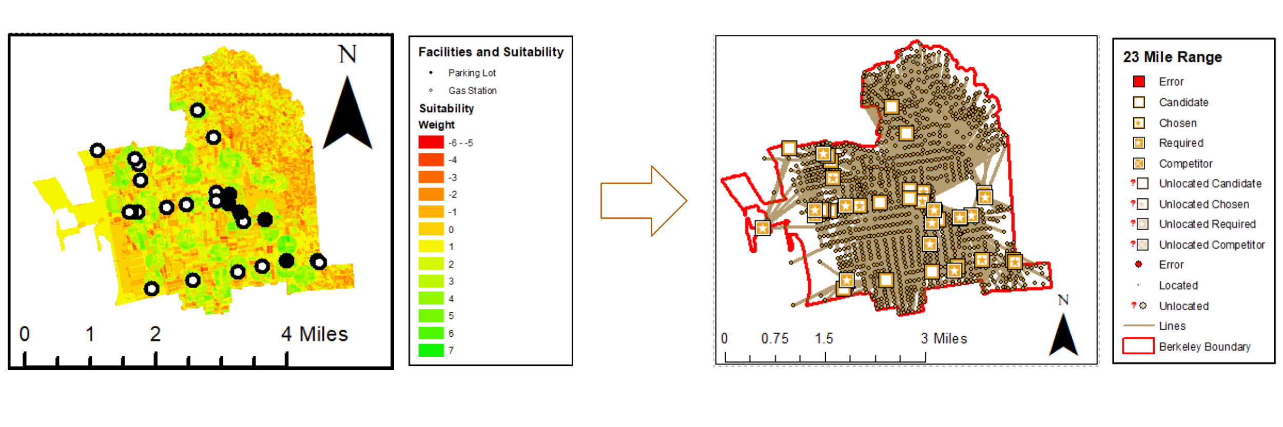
Step I: Load facilities from Google Earth Pro (KML to Layer). Populate parking facility metadata, inputting time open, parking fee, available spaces in attribute table. Calculate capacity.

Step II: Spatial Join final suitability map with candidate facilities to calculate facility weight.

Step III: New Maximize Capacitated Coverage. Load Candidates and Required locations into Facilities with appropriate weights and capacities. Load census block centroids as demand points weighted by number of persons.

Step IV: Set impedance parameters and solve for stations.

Equations

Capacity:

• Formula: Chargers * Time available / ( Charging time / # Plugs )
• Charging time: 2 hours (full battery), 0.23 hours (23 mi. charge)
• Time available for charge: opening hours:
  • assume chargers are always open
  • assume gas stations are always open
  • parking lots have defined hours open
• Plugs: 2 plugs / charger
• Chargers: # spaces / 2
  • Assume: gas stations: 8 spaces; existing chargers: 2 spaces

Weight:

• Formula: 7 + Relative price + Suitability weight
• Relative price: ( Prices / Lowest price ) * -1
• 7: sum of negative weights is 6, and weight must be greater than or equal to 1, thus the choice of 7.

Additional Graphs and Media

3D Slope Analysis Procedure

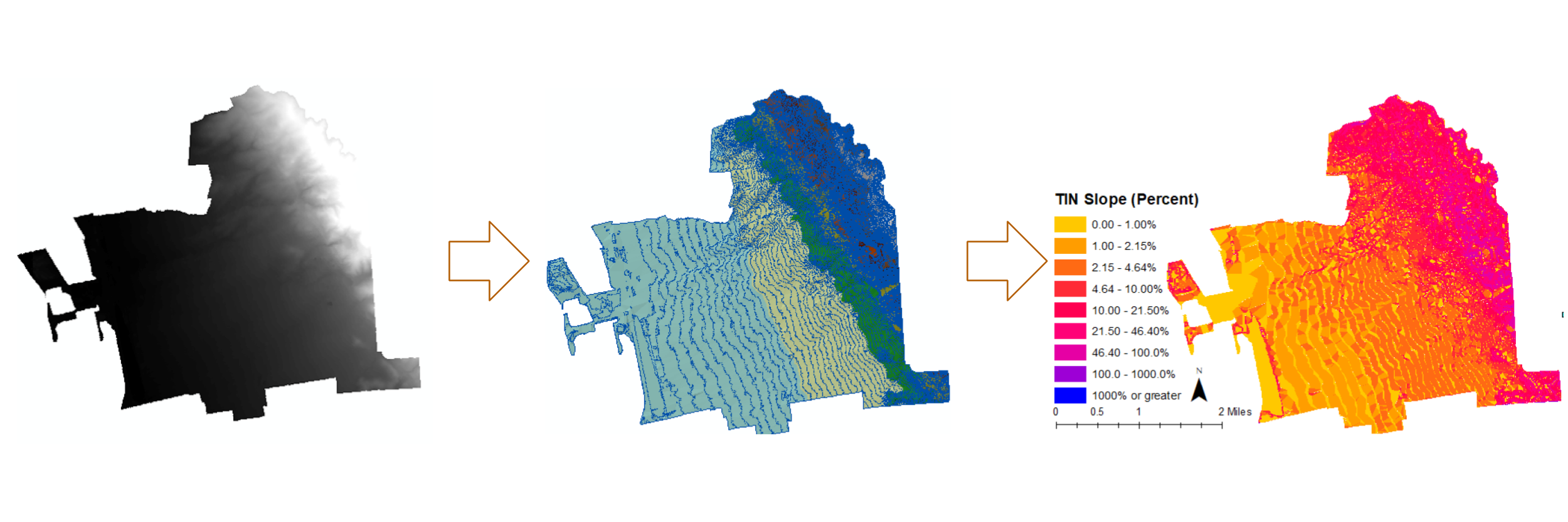
Step I: Clip DEM to Berkeley bound.

Step II: Compute Contours (10m) from DEM.

Step III: Compute TIN from Contours.

Step IV: Clip TIN to Berkeley bound.

Step V: Calculate Surface Slope from clipped TIN.

Step VI: Dissolve surface slope by slope code.

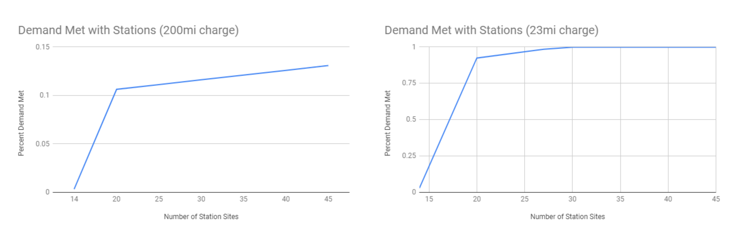
Effects of New Charging Stations on Demand Met