Computer Vision

Overview

Computational Photography is an emerging new field created by the convergence of computer graphics, computer vision and photography. Its role is to overcome the limitations of the traditional camera by using computational techniques to produce a richer, more vivid, perhaps more perceptually meaningful representation of our visual world.

The aim of my study was to find ways in which samples from the real world (images and video) can be used to generate compelling computer graphics imagery. I learned how to acquire, represent, and render scenes from digitized photographs. Several popular image-based algorithms were presented, with an emphasis on using these techniques to build practical systems. This hands-on emphasis is reflected in the programming assignments, in which I had the opportunity to acquire my own images of indoor and outdoor scenes and develop the image analysis and synthesis tools needed to render and view the scenes on the computer.

Topics Covered

• Cameras, Image Formation
• Visual Perception
• Image and Video Processing (filtering, anti-aliasing, pyramids)
• Image Manipulation (warping, morphing, mosaicing, matting, compositing)
• Modeling and Synthesis with Visual Big Data
• High Dynamic Range Imaging and Tone Mapping
• Image-Based Lighting
• Image-Based Rendering
• Non-photorealistic rendering

Selected Projects

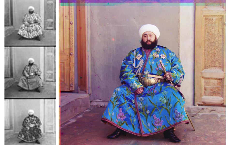
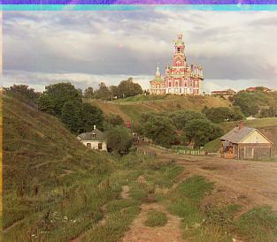
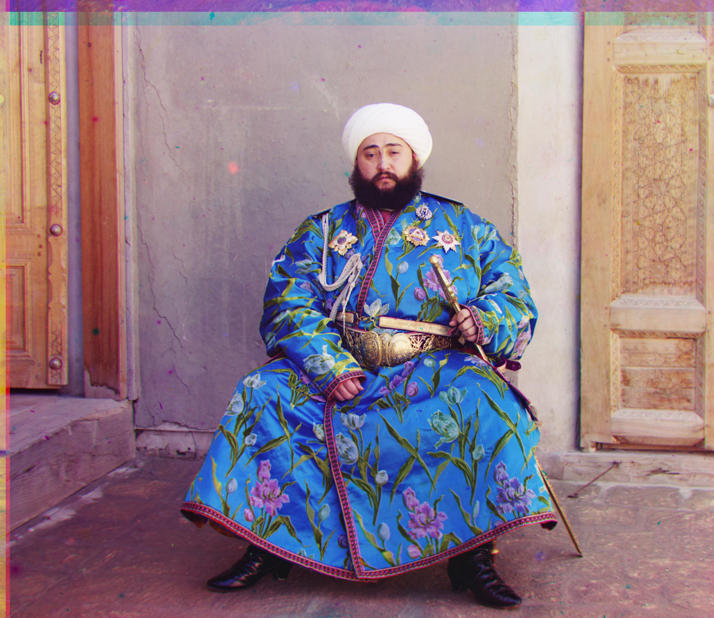
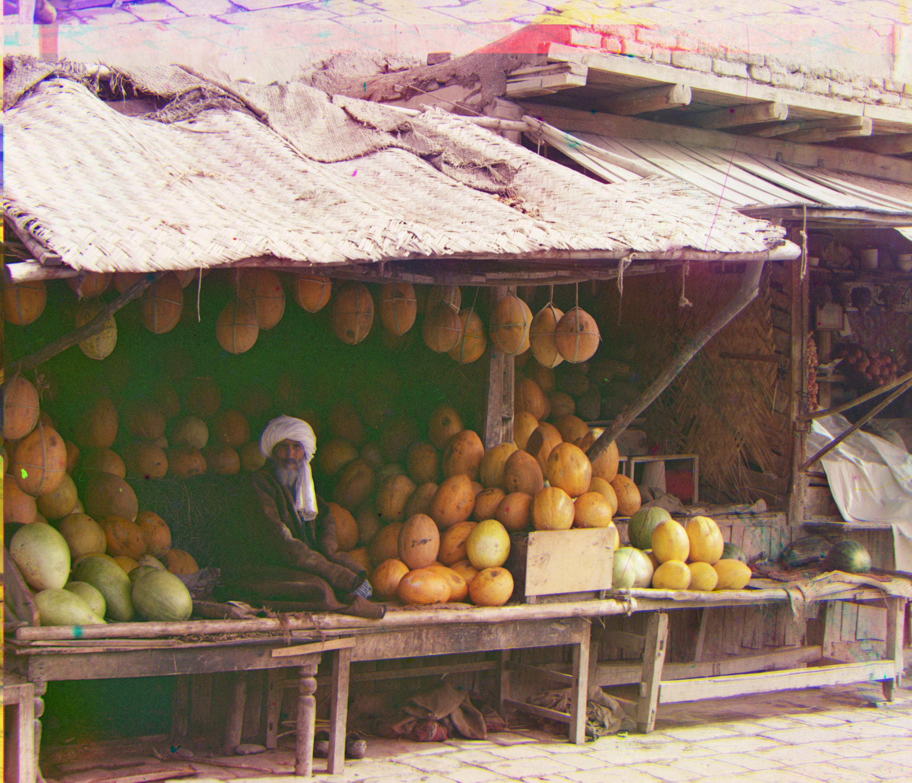
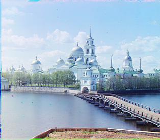
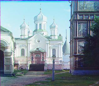
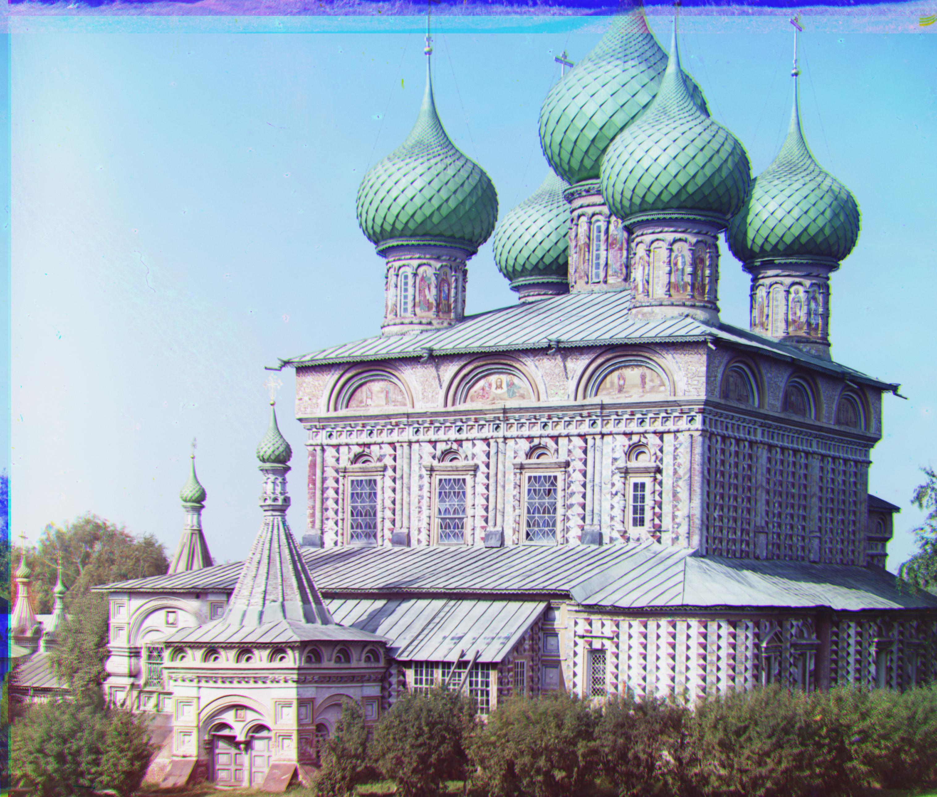
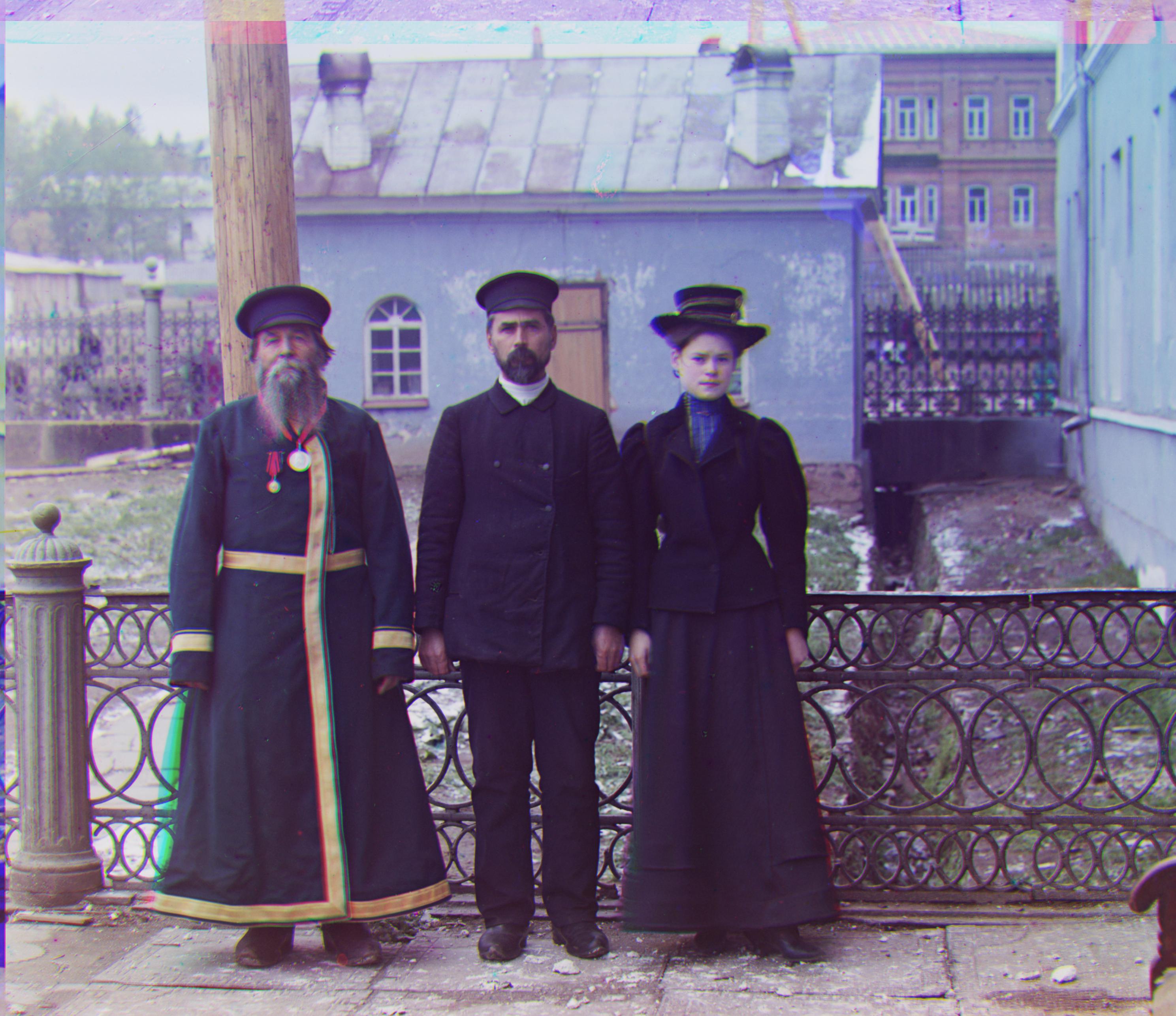
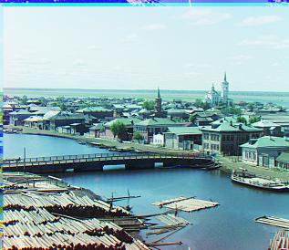
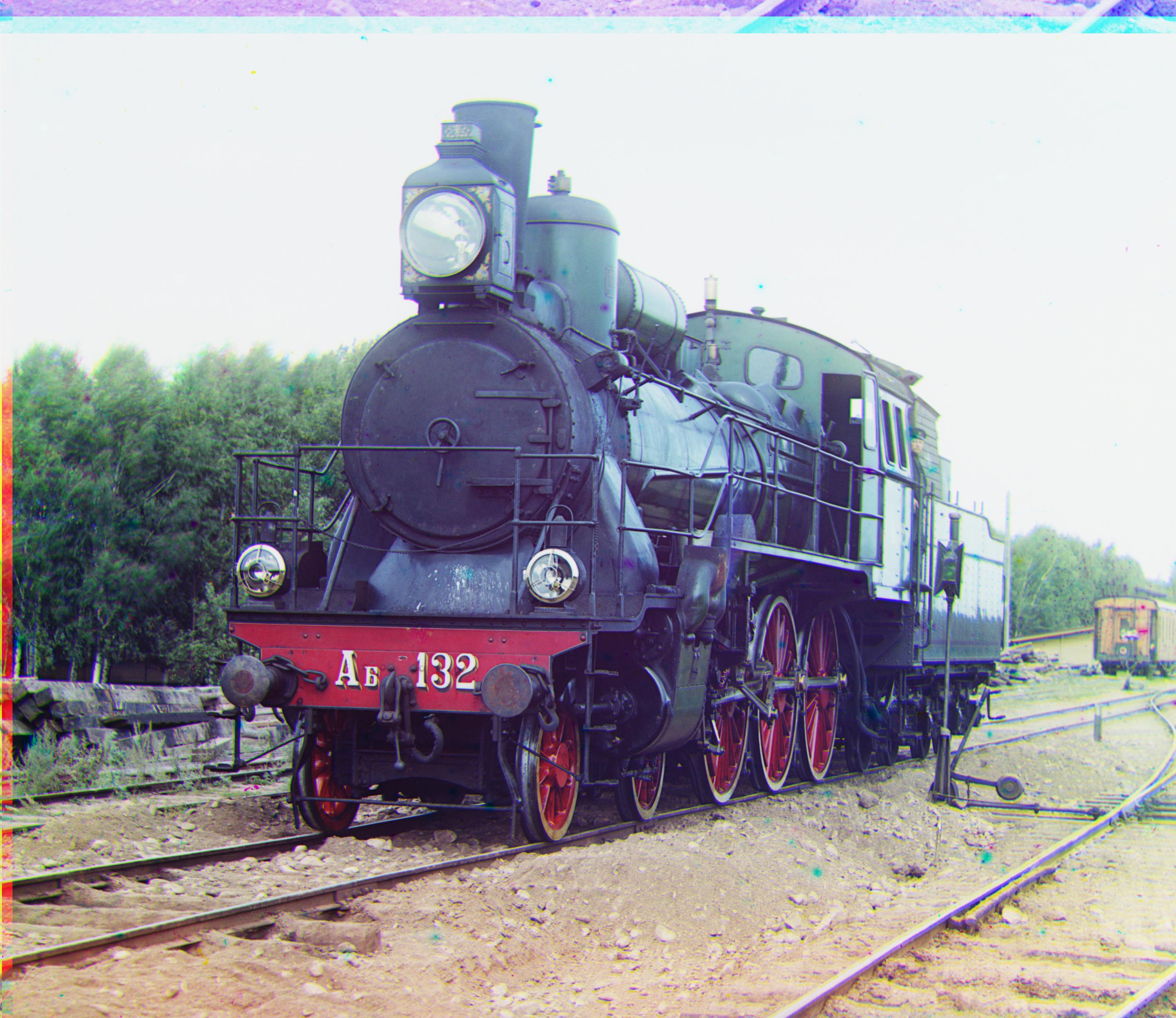
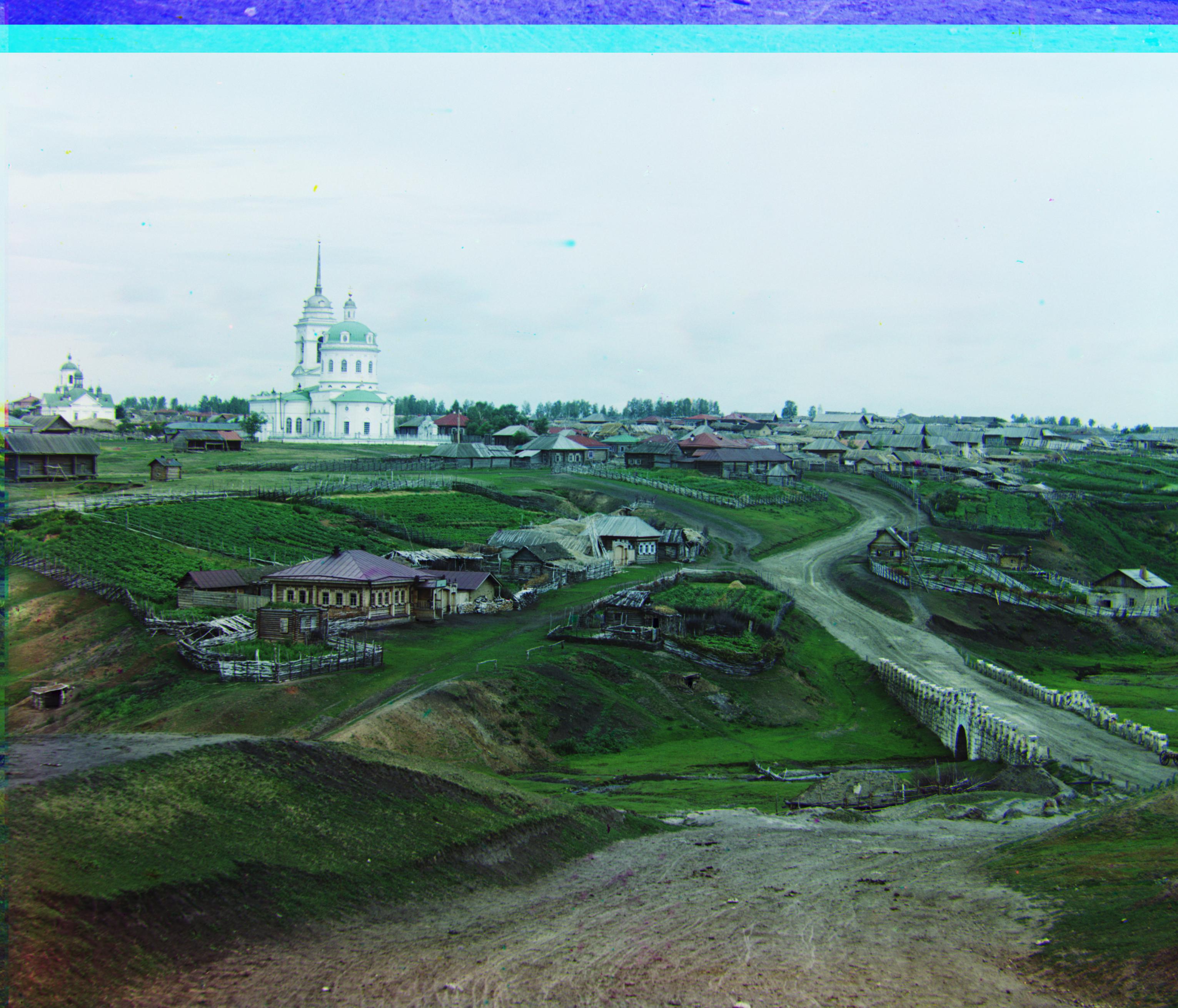
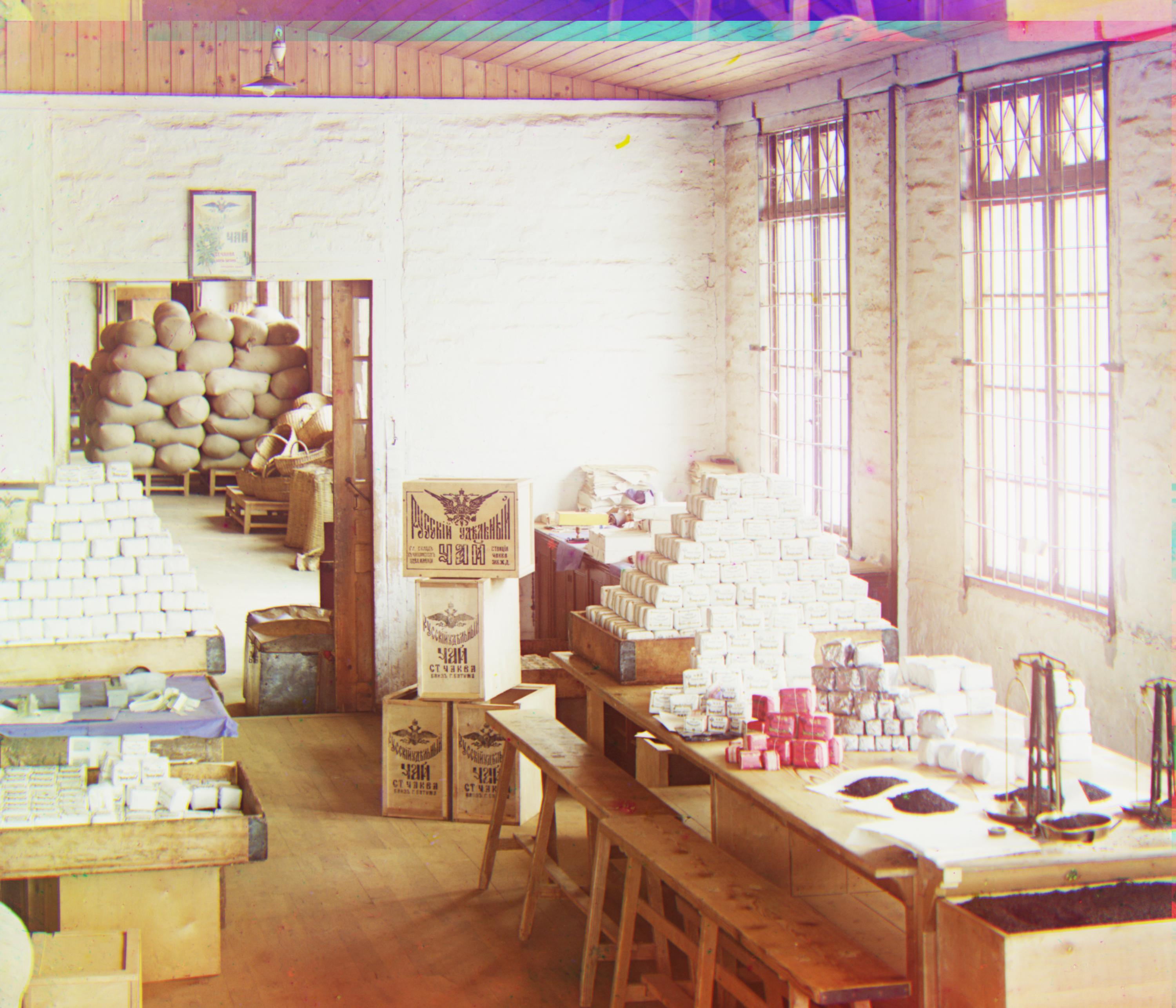
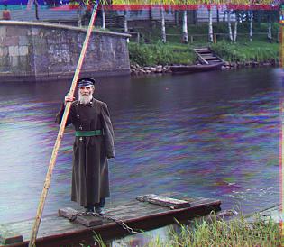
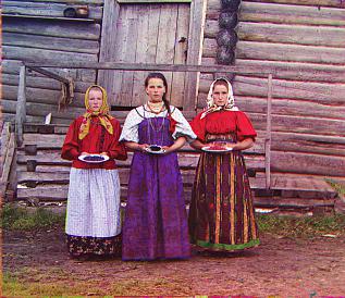
Project: Colorizing the Prokudin-Gorskii photo collection

Overview

The goal of Project 1 is to take the Prokudin-Gorskii glass plate images and implement a red-green-blue algorithm in order to produce a colored version of the images. The algorithm is responsible for merging the three RGB-filtered images in order to produce a final aligned colored image.

Algorithms

In order to align the images together, I searched over a window of possible displacements, and find the displacement with the best results. I used normalized cross-correlation (NCC) to determine which displacement gave me the best results. To reach results faster, I implemented an image pyramid to recursively search through the image for the best displacement window. The image pyramid represents the image at multiple scales and then proceeds from the smallest image to the largest image to update the estimated window of displacement. Lastly, I used a for loop to go through each image in the data file, and applied the separating RGB, finding displacement, and aligning functions. What I found interesting was that the images were more accurately aligned after cropping 10% of the border of each image.

Resulting Images

Project: Lightfield Camera

Overview

This project addresses depth refocusing. Depth refocusing refers to the changing of the focus depth in images after them being taken, by using multiple photos of the same object. We shift and average the images together in order to effectively refocus the image. I used images from the Stanford Light Field Archive dataset, which provides images taken with a grid of cameras.

Algorithms: Implementing Depth Refocusing

Generally when we move the camera in pictures, objects that are far away do not move as much as objects closer to us. Therefore, when we average all the images in the dataset, we get sharp far-away objects, and blurry close-by objects. To avoid this, we center the image around a center image, and then we shift the images by the depth-focus adjustment amount of our choice (I chose values [-3, 1]). This allows us to focus on objects at different depths.

Resulting Images

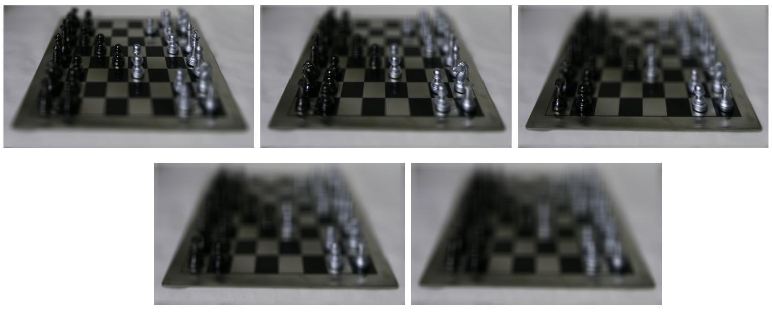
Here are the images depth-refocused at different centers ([-3, 1] by steps of 1):

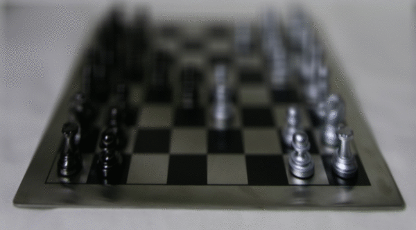
Here is an animation of the image with depth-refocused:

Algorithms: Implementing Aperature Adjustment

We average a large number of images surrounding the optical axis on the grid to determine ranges that represent aperature sizes. As the aperature gets bigger (on a camera, lets in more light), a larger range of images contribute to the average image. Conversely, as the aperature gets smaller (lets in less light on a camera), the range of images contributing to the average image is also smaller.

Resulting Images

Here is the image with the largest aperature:

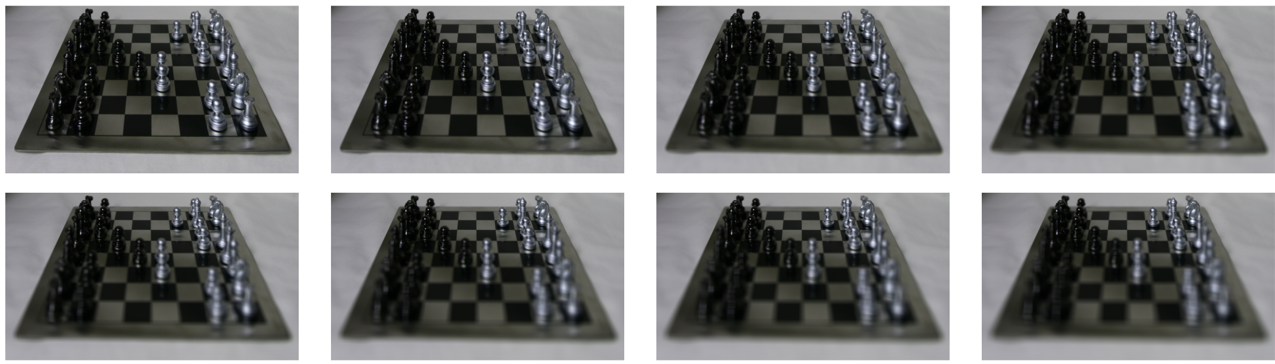
Here are the images with the aperature adjusted:

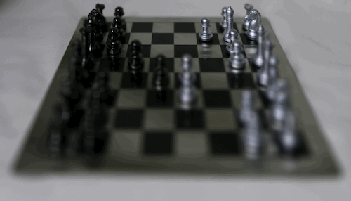
Here is an animation of the image with aperature adjusted:

Here is another image from the Stanford Light Field Archive with the largest aperature:

Here is an animation of the image with aperature adjusted:

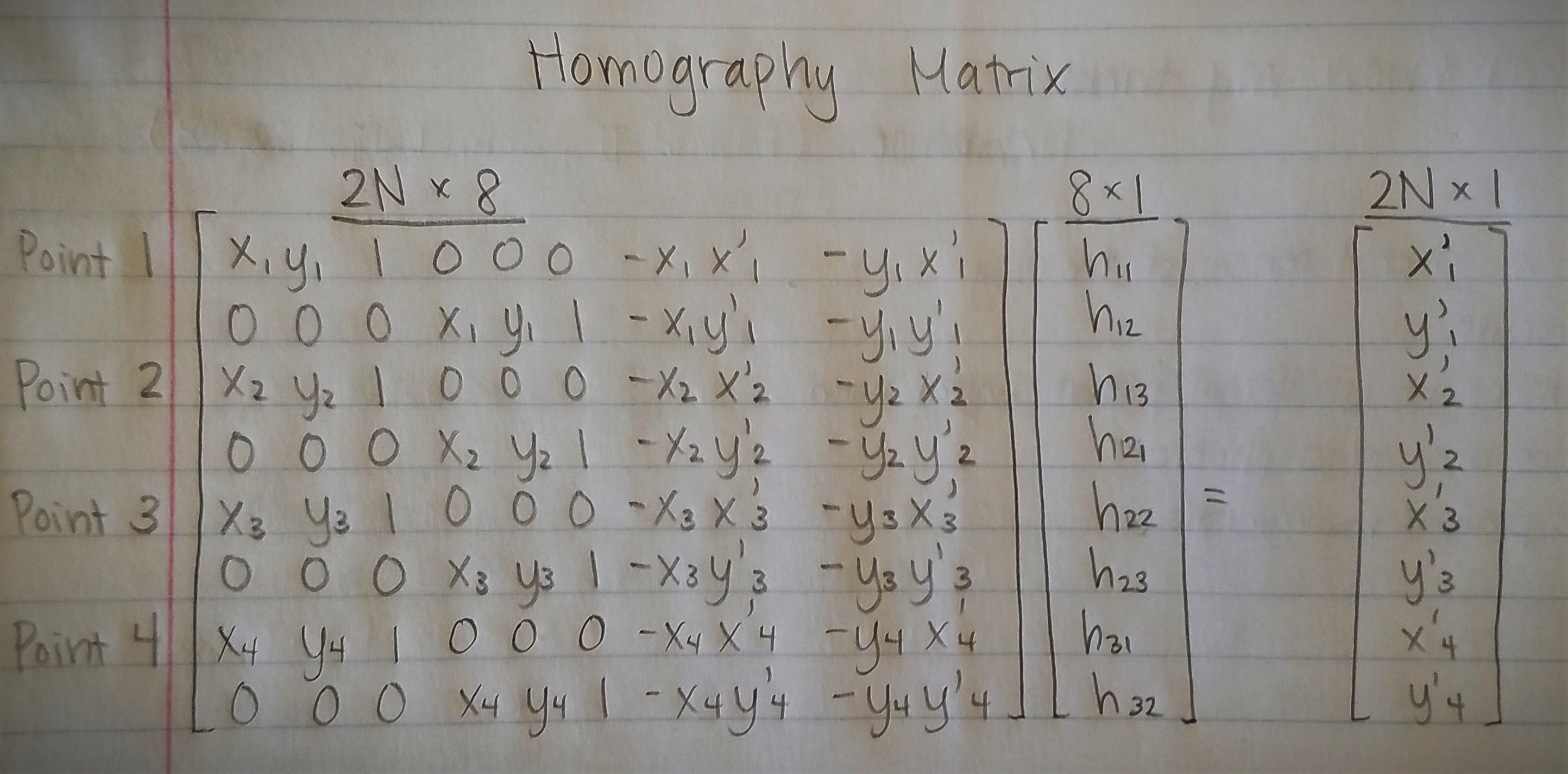
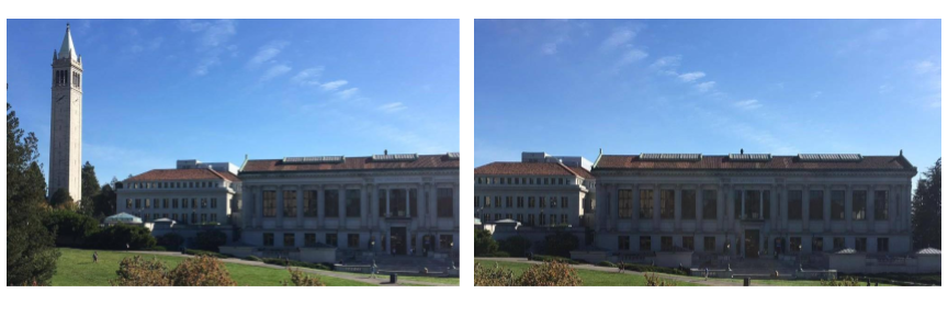
Project: (Auto)-Stitching and Photo Mosaics

Overview

We can stitch 2-D images to create a panorama by taking multiple images along an axis and then defining homographies to warp from one image to another.

Recover Homographies

We use at four points of correspondency to create a usable 3x3 homography matrix with 8 degrees of freedom.

Warping Images

After computing the homography matrix, we can warp the images. We use one image as the center and warp the other images towards the center image. We pipe the corners of the image through the homography matrix, thus giving us the shape of the warped image. Then we use the inverse of the homography matrix to find the points on the original image that map to the warped image.

Rectifying Images

After warping the images, we rectify the images by picking a feature point in the image, and then changing the point of view of that feature point to be frontal.

Blending Images

We can warp the images to align with the center image, and use average weighting and alpha blending to remove any strong edges. The center image has an alpha of 1, and we continuously decrease the alpha value (linearly) as we progress further from the center image.

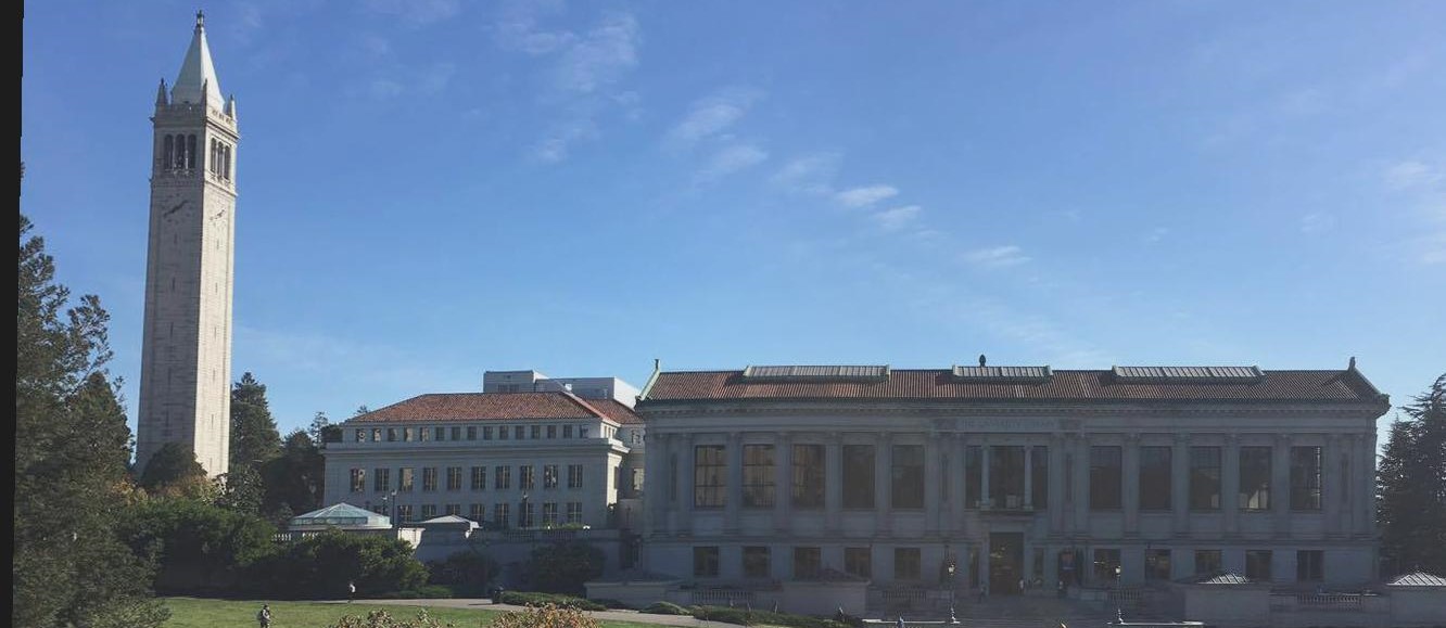
Here are the original images, that I will blend after:

Here are the images blended together:

Auto-Stitching Images

In this part of the project, we implement autostitching, as opposed to manual stitching in the previous part.

We take the original photos from above, and we implement four different types of point detectors:

1. Harris Intersect Point Detector
2. Adaptive Non-Maximal Suppression
3. Feature Descriptor Pairs
4. RANSAC

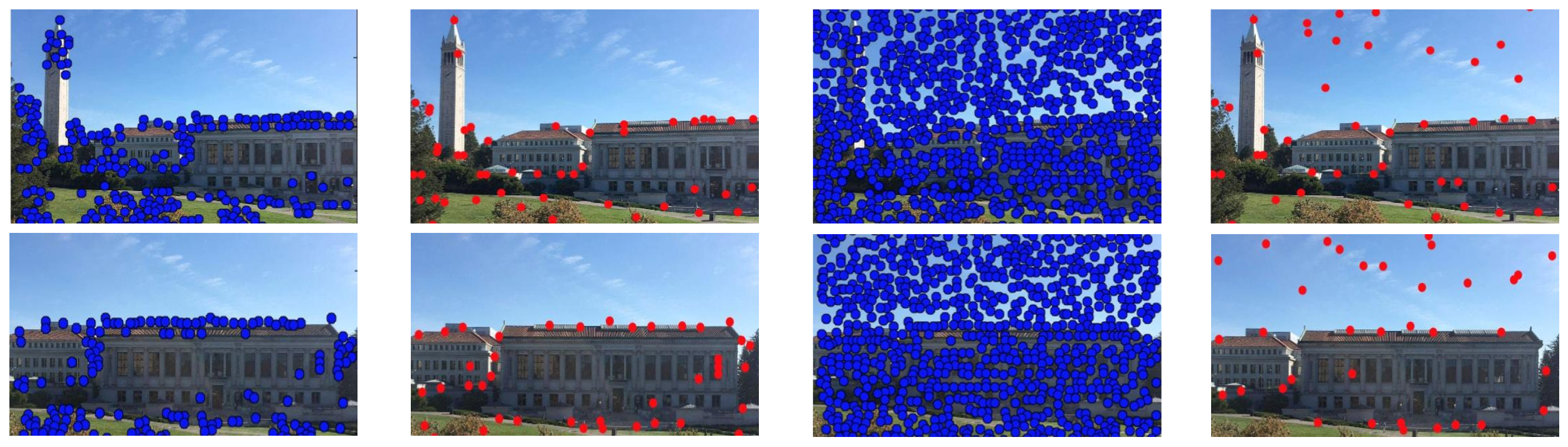
Here is the resulting auto-stitch of the image:

Conclusion

These are just some of the many projects I did during my independent study. I want to thank Professor Efros for everything I learned and for creating all these fun and interesting projects!